Fitting Cycles to a Time Series

I had a dataset with monthly prices going back to 2017. The kind of data that grows fast and oscillates — big peaks, big crashes, roughly every few years.

I wanted to see if I could model it with a single equation.

Power law for the trend

First, fit a power law to capture the overall growth:

price = A * t^a

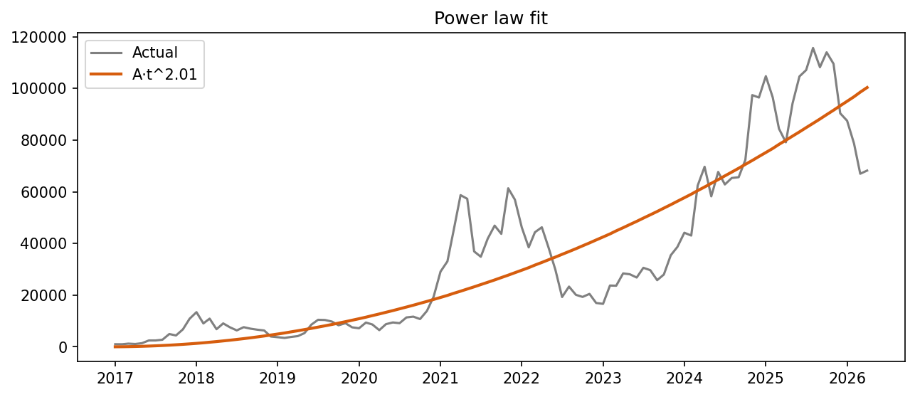
On a log scale, the fit is easier to judge across the full range:

It found t^2 — quadratic growth. Captures the trend, ignores the cycles.

The residual

Subtract the power law and look at what's left:

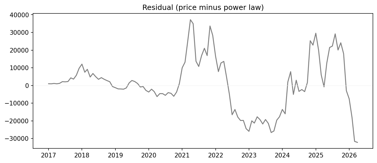
Clear oscillation, roughly every 3-4 years. But the amplitude grows over time — a regular sine wave can't capture that.

Multiply instead of add

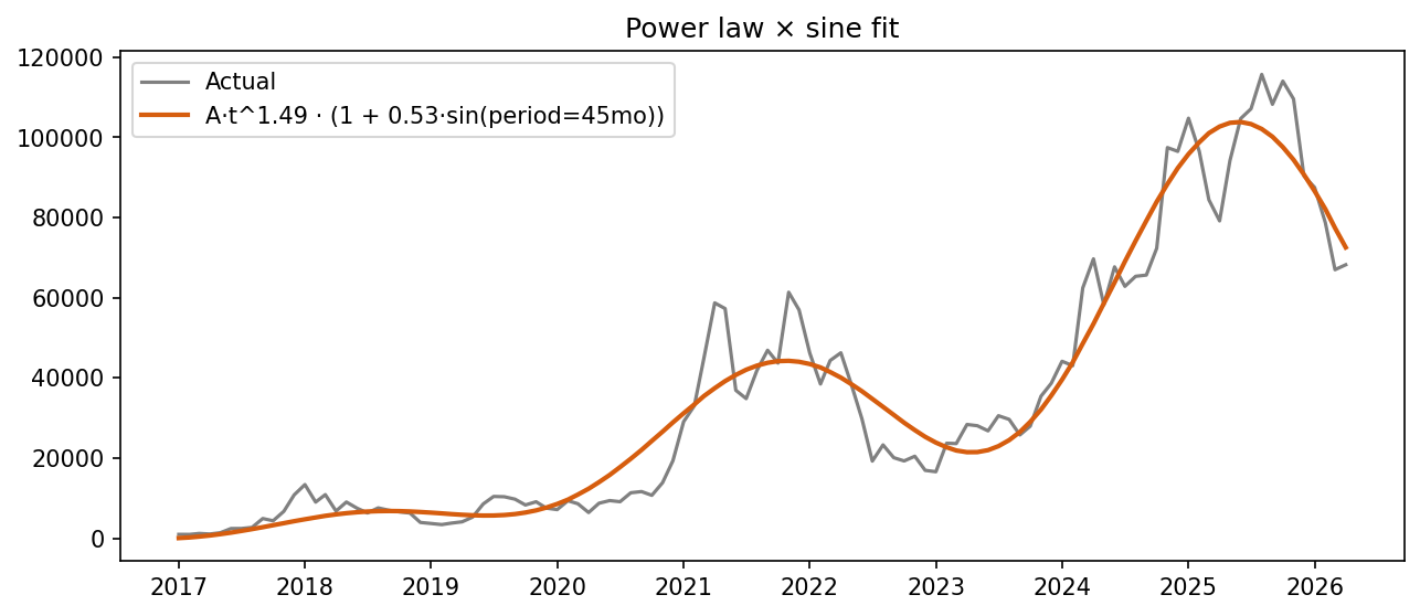
Instead of fitting trend and cycles separately, multiply them:

price = A * t^a * (1 + B * sin(2π * f * t + phase))

The power law handles the growth. The sine modulates it up and down. Because they're multiplied, the swings scale naturally with the price level.

def model(t, A, a, B, f, phase):
    return A * t ** a * (1 + B * np.sin(2 * np.pi * f * t + phase))

best_popt, best_err = None, np.inf
for period in range(6, n, 2):
    fg = 1 / period
    try:
        popt, _ = curve_fit(model, t, prices,
                            p0=[1.0, 2.0, 0.5, fg, 0.0], maxfev=10000)
        err = np.sum((prices - model(t, *popt)) ** 2)
        if err < best_err:
            best_err, best_popt = err, popt
    except RuntimeError:
        continue

One equation, five parameters. The fit found a ~45-month cycle with ±53% modulation around a t^1.5 growth curve:

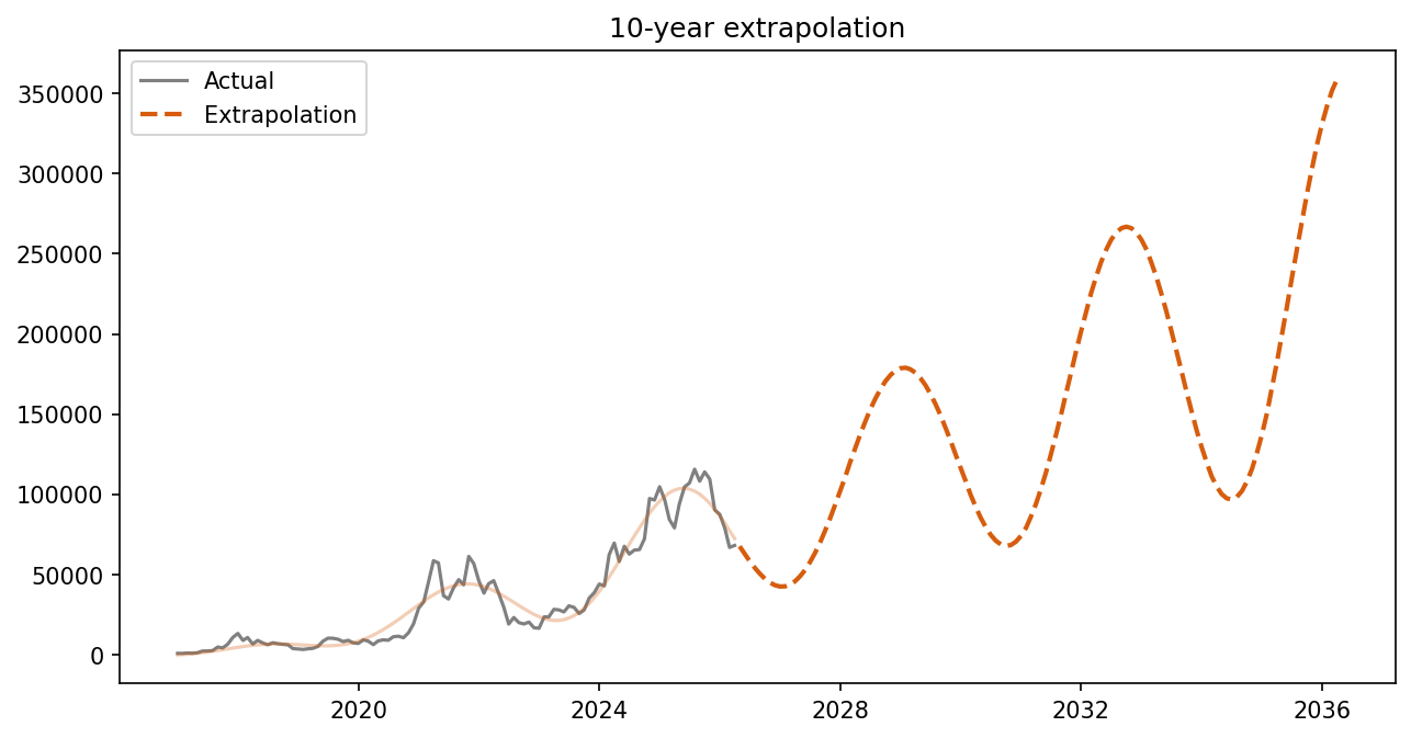
Extrapolation (for fun)

Pure pattern extrapolation — not a prediction:

What I learned

• Separating trend from cycles is key. Trying to fit everything at once doesn't converge well.
• Multiplying instead of adding is the right way to combine growth with oscillation when the amplitude scales.
• Five parameters can go a long way.
• scipy.optimize.curve_fit is a workhorse.