String art — teaching a greedy algorithm to draw with thread

The solver and code are mine; this write-up was drafted by Claude.

My cousin has been making string art — the kind where you hammer a few hundred nails around a frame and wind a single black thread back and forth until a face appears out of the chaos. It's mesmerising to watch. And of course the part my brain latched onto wasn't the hammering, it was: how would you compute which nail to go to next?

So I built a tiny solver. The whole thing is one short Python file; the interesting bit is a single function. This post is about that function.

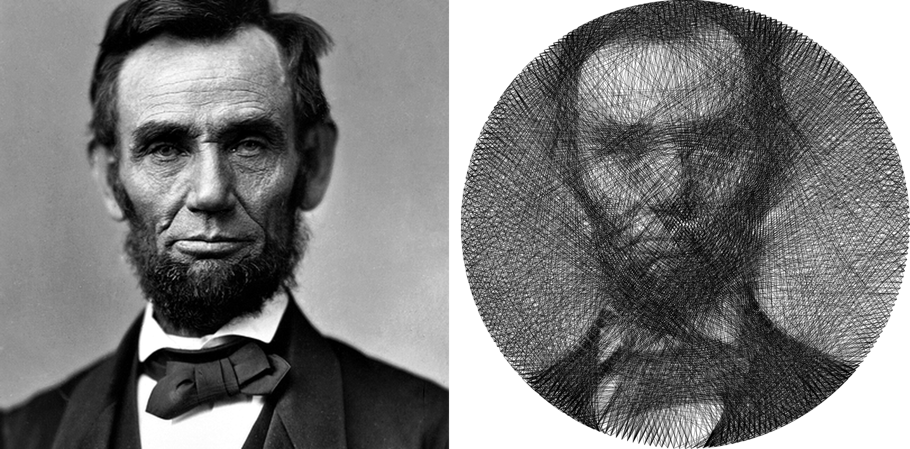
The reframe

Physically, string art is a continuous thread hopping between pins on the edge of a frame. Each straight run of thread is a chord — a line between two pins — and it deposits a thin, semi-transparent streak of black wherever it crosses.

Turn that around and it becomes an image problem. Start from the target picture as a map of "how dark should each spot be". Every chord you add darkens a line of pixels. The question is just: which chord, added next, best closes the gap between what you've drawn and what you want?

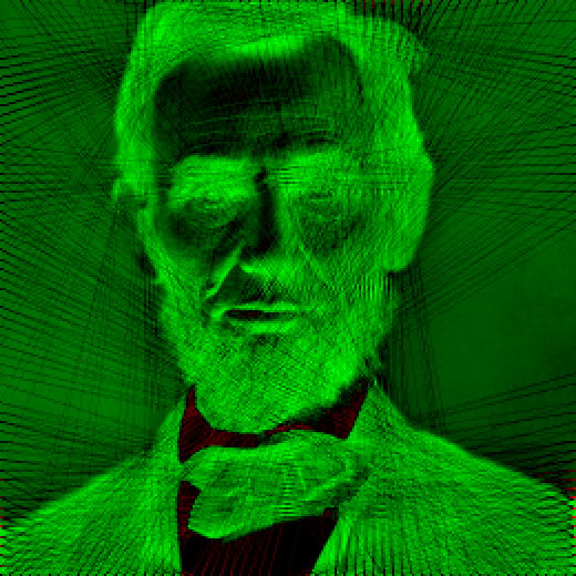
That gap has a name in the code: the residual. It starts as the target (1 = full black, 0 = white) and every thread you lay subtracts a little darkness along its path. Green where you still owe thread, red where you've overdone it:

The greedy idea

At each step:

1. From the pin where the thread currently sits, look at every chord to every other pin.
2. Score each one by the average leftover darkness along the pixels it would cross — i.e. how much of it lands where the image still wants black.
3. Take the best chord, "lay" it by subtracting its darkness from the residual, and move to its far pin.
4. Repeat until no chord helps, or you hit a line budget.

The constraint that makes it feel like real string art: each new line starts where the last one ended. It's one continuous thread, not a free-for-all of disconnected segments.

def solve(residual, pins, opacity, max_lines):
    h, w = residual.shape
    flat = residual.reshape(-1)               # image as a flat darkness map
    N = len(pins)

    # for every pair of pins, precompute which cells that chord crosses
    pix = {(a, b): line_pixels(*pins[a], *pins[b], w, h)
           for a in range(N) for b in range(a + 1, N)}
    pix |= {(b, a): v for (a, b), v in pix.items()}

    def score(c):                             # avg leftover darkness along the chord
        p = pix[c]
        return flat[p].sum() / p.size

    # start with the single best chord anywhere
    segments = [max(pix, key=score)]
    flat[pix[segments[-1]]] -= opacity

    placed = set()
    for _ in range(max_lines):
        src = segments[-1][1]                 # continue from the last pin
        nxt = max((t for t in range(N) if t != src and (src, t) not in placed),
                  key=lambda t: score((src, t)))
        if score((src, nxt)) <= 0:            # nothing left worth darkening
            break
        segments.append((src, nxt))
        flat[pix[(src, nxt)]] -= opacity      # lay the thread
        placed |= {(src, nxt), (nxt, src)}
    return segments

(Lightly trimmed from the repo — I've dropped the debug prints and a couple of residual dumps.) Two small things carry most of the weight:

• Precomputing the pixels each chord crosses. With a couple hundred pins there are tens of thousands of possible chords, but they never move — only the residual underneath them changes. Compute them once, and scoring a chord becomes a single sum() over a precomputed index array.
• flat[pix[...]] -= opacity. That one subtraction is the entire feedback loop. Lay a thread, the residual under it drops, and those pixels stop attracting more thread. The image fills itself in.

And it stays cheap: because the next line is anchored at the pin the thread already sits on, each step only scores the ~N possible next pins — linear in the pin count, not the O(N²) chords you'd weigh if a line could start anywhere. With the pixels precomputed, that's just N small sums per step.

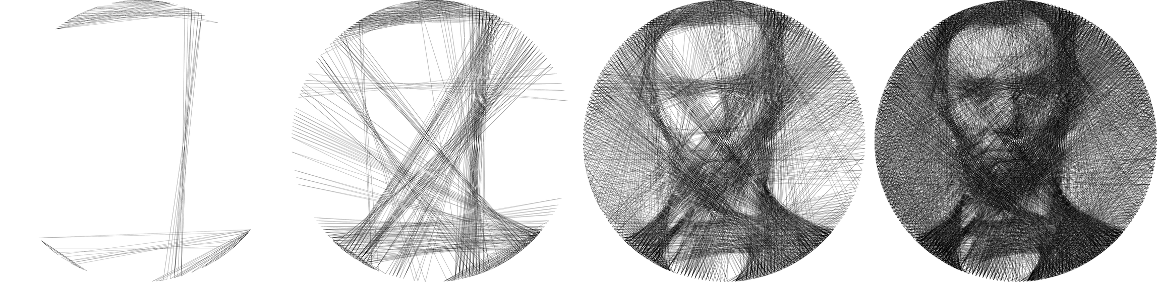
Watch it converge — 120 lines, 500, 1,500, and the full ~2,800:

Or watch it build the whole thing, one thread at a time — hit play, or drag to scrub. It's the pin path replayed on a canvas (~14 KB of data), not a video:

Honest millimetres

One thing I wanted from the start: the rendered preview should look like what you'd actually wind on the wall, not a stylised approximation. So the frame and the thread are described in real units — a 300 × 300 mm frame, a 0.12 mm thread — and those measurements drive the picture.

The renderer leans on that. A 0.12 mm thread is far thinner than a single output pixel, so instead of faking thinness with transparency, every thread is drawn full opaque black on a supersampled canvas (where it still spans at least a pixel) and then downscaled. The sub-millimetre thread becomes genuine grey by coverage — the same way your eye averages it out from across the room. The solver's opacity is the matching idea on the input side: the fraction of a grid cell that real thread actually covers, thread_mm / (frame_mm / grid). Thinner thread or a bigger frame makes each line count for less, and the solver reaches for more of them — exactly as it would in reality.

Wind that thread on that frame, and the output should be a faithful preview, not a flattering one.

Pins don't have to be a circle

The classic look is a circle of nails, but pins is just a list of points — the solver doesn't care about the boundary's shape. So I gave it a few: a circle, a flat-top triangle, a five-pointed star. Same Lincoln, same solver, different frames:

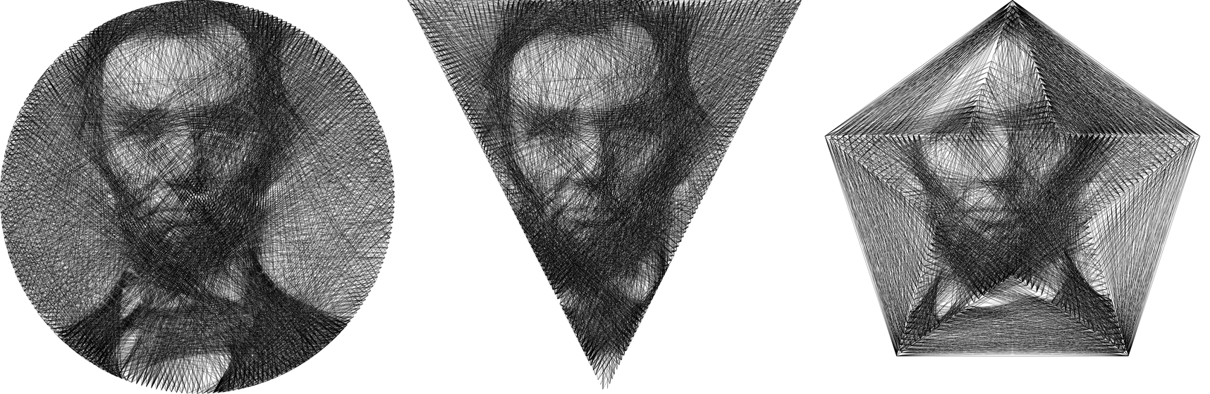
The star is my favourite — the concave notches force long chords straight across the middle, and the face shows up anyway.

Simple on purpose

I started dumb on purpose — just to see what the most naive version would give. One continuous thread, never cut, hopping from pin to pin; pick the next pin by the mean of the residual values along the line, and move on. No restitching of disconnected segments, no global optimiser second-guessing earlier moves.

Because it's a single greedy walk, the winding order comes out for free — the sequence of pins is the answer, with no extra step to turn a pile of chords back into one continuous thread. And honestly, the result surprised me. Good enough for me.

What's out there

A short, sourced map of how this gets solved — I'm not an expert, so this is what I could actually find.

The modern circular-nail portrait traces to artist Petros Vrellis, A New Way to Knit (2016) — 200 pins on a round frame, one continuous thread. He didn't publish his method; the open-source solvers that followed reverse-engineered it as a greedy loop.

Most of that open-source work is laid out in Roy Hachnochi's writeup, which compares three approaches: a naive greedy optimiser (each step, add the line that reduces the error most), a linear-regression formulation (solve A·x = b over all chords — least squares, treating overlapping threads as if they add linearly), and a binary-linear hybrid that pairs greedy selection with the linear formulation through a fast per-step update. On the input side, the tricks it documents are negating the image (thread = black) and an importance/weight map to push detail where it matters — not edge detection or fancy filtering.

The main academic treatment is Birsak, Rist, Wonka & Musialski, String Art: Towards Computational Fabrication of String Images (Eurographics 2018): a discrete optimisation that turns a picture into a connected graph of strings, paired with a robot that winds it physically. Their code is on GitHub.